Blog Post:

Moving Average vs. Exponential Smoothing: Choosing the Right Real-Time Data Filter

Home » Blog » Moving Average vs. Exponential Smoothing: Choosing the Right Real-Time Data Filter

Often when working with real time data, a programmer needs to smooth out a recent set of live data points to make decisions based on the incoming data. The simplest way to do this conceptually is to use a windowed moving average. The basic method involves taking a record of the past N data points and recalculating the mean every time a new data point comes in. The formula for a moving average is shown below, where N is the window size:

$\bar{s}_{t} = \frac{1}{N} \sum_{i=0}^{N-1} x_{t-i}$

This method is very intuitive, has predictable behavior, and is easy to explain to non-technical personnel. However, there are some drawbacks to this approach:

Can require a large amount of memory for recording the last N data points.
- For a true moving average, the program needs to keep a buffer of the last N data points, which can very quickly fill up program memory if N is exceptionally large, especially in an embedded application with constrained memory resources.
May involve dynamic memory allocation if the window size needs to be changed at runtime.
- If the window needs to change at runtime, the buffer for storing the last N data points needs to grow or shrink to adapt to a given window size. This typically requires dynamic memory allocation, which could add complexity to an embedded project.

Alternative Approach: Exponential Smoothing

One alternative to a moving average is Simple Exponential Smoothing (sometimes called an Infinite Impulse Response Filter or a Single Pole Low Pass Recursive Filter). The basic method can be described by a recursive relation:

$\alpha \in [0,1]$

$s_t = (1 - \alpha)\cdot s_{t-1} + \alpha\cdot x_t$

Where $s_t$ is the new smoothed value, $s_{t-1}$ is the previous smoothed value, and $x_t$ is the latest data point. Solving for non-recursive relation, we can get:

$s_t = \alpha \cdot \big( x_t + (1-\alpha)\cdot x_{t-1} + \cdots + (1-\alpha)^{t-1}\cdot x_1 + (1-\alpha)^t\cdot x_0 \big)$

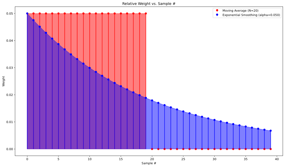
From this formula, we can make the observation that this is just a specific case of a weighted average, where the more recent data points are weighted higher than older data points, and as successive values are calculated, the older data points “decay” to the point that in practice the data becomes negligible to the newly calculated smoothed value. This behavior roughly approximates a moving average, albeit with uneven weighting of the data points. This weighting can be visualized by graphing the impulse response of both approaches.

To illustrate the similarities in another way, we can get a recursive formula for the true moving average by subtracting two successive calculations of the moving average.

$\bar{s}_{t} - \bar{s}_{t-1} = \frac{1}{N} \sum_{i=0}^{N-1} x_{t-i} - \frac{1}{N} \sum_{i=0}^{N-1} x_{t-1-i}$

$= \frac{1}{N} x_t + \frac{1}{N} \sum_{i=1}^{N-1} x_{t-i} - \frac{1}{N} \sum_{i=0}^{N-2} x_{t-1-i} - \frac{1}{N} x_{t-N}$

$= \frac{1}{N} x_t + \frac{1}{N} \sum_{i=1}^{N-1} x_{t-i} - \frac{1}{N} \sum_{j=1}^{N-1} x_{t-j} - \frac{1}{N} x_{t-N}$

$= \frac{1}{N} x_t - \frac{1}{N} x_{t-N}$

$\bar{s}_t = \bar{s}_{t-1} + \frac{1}{N} \big( x_t - x_{t-N} \big)$

If we compare this result to a rearranged exponential smoothing relation, we can see the similarity:

$s_t = (1 - \alpha) \cdot s_{t-1} + \alpha \cdot x_t$

$s_t = s_{t-1} + \alpha \cdot (x_t - s_{t-1})$

Both $\alpha$ and $\frac{1}{N}$ are numbers between 0 and 1, so the exponential smoothing is functionally a moving average where instead of subtracting an oldest measurement ( $x_{t-N}$ ), instead we use the previous estimate to find a difference for the next estimate. The advantage here is that the exponential smoothing formula allows the calculation to forego keeping track of anything but the previous smoothed value and the new data point. This means no N-length buffer to keep track of data, and as an added bonus, the window of the moving average can be adjusted on the fly without needing to allocate memory dynamically.

Analogy between $\alpha$ and N

For a true “apples to apples” comparison, we need to match the different constant parameters for each approach. This means finding some sort of equivalence between N in the moving average and in the exponential smoothing. This process is largely arbitrary, but with a couple assumptions, we can make a reasonable comparison. We can start by looking at the non-recursive formula from before, noticing that the weight of any data point in the overall formula is multiplied by $(1 - \alpha)$ every iteration. This means the weight of a data point collected iterations ago will look like:

$\alpha (1 - \alpha)^i$

Here we assume that if the formula is to behave *roughly* like a moving average of size N, the Nth term of the series should be an arbitrary small percentage of the initial data point. In other words, the Nth previous sample should decay to a small percentage of what the term was initially, and as a result, any of the samples older than the Nth would be even smaller, and thus negligible to the overall calculation. For our example, let’s say 10% is our target decay for the Nth term. This gives:

$(1 - \alpha)^N = 0.10$

Rearranging for $\alpha$ , we get:

$\alpha = 1 - 0.10^{\frac{1}{N}}$

This gives us a way to get from a given desired N, and consequently, a way to get a roughly equivalent exponential smoothing filter for a given moving average. It’s worth noting that the choice of 10% is arbitrary here, and varying that choice can result in a wide range of different behaviors for the exponential smoothing,

Graphical Comparison

To visualize the difference in behavior of the two approaches, we can operate both on the same test data and graph the results at each time step. With the data of a noisy cosine pattern, we get the following graphs:

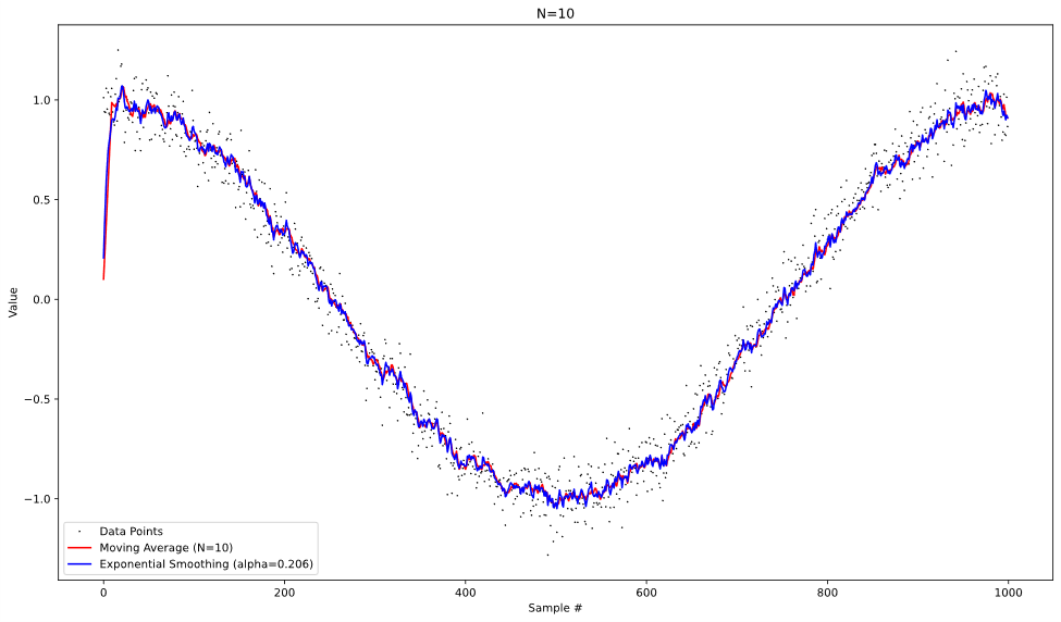
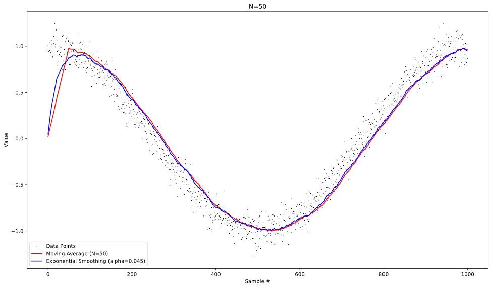
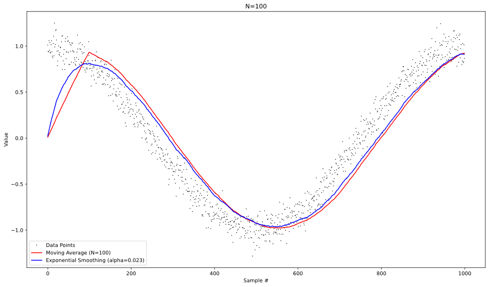
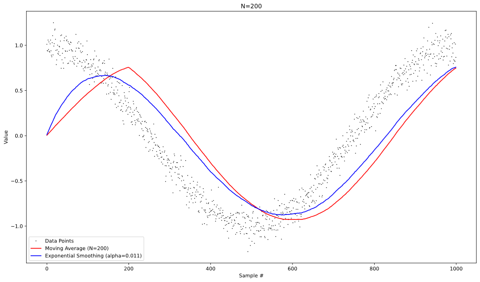
From looking at these plots, we can see that both approaches behave similarly when operating on the noisy data, albeit with more lag introduced in the moving average at higher values of N. It’s also worth noting that the moving average is slightly better at reducing the random noise from the data, especially at lower values of N.

Summary

In comparing these two approaches, we can see distinct advantages for both approaches. The moving average filter is much more intuitive to understand and can be explained clearly even to non-technical people. It also can reduce noise from the data more effectively. The exponential smoothing technique, on the other hand, has an extremely simple recursive implementation, and does not require a large amount of memory to work effectively. Also, the exponential smoothing can be reconfigured on the fly without allocating new memory by changing $\alpha$ , while a moving average would need to change the size of its buffer dynamically to do the same. When working with embedded systems with memory constraints, it is worth considering exponential smoothing as an alternative to a moving average.

	Moving Average	Exponential Smoothing
Memory Usage	Moderate (N data points)	Low (single data point)
Software Complexity	Moderately Complex	Extremely simple
Runtime Window Adjustment	Dynamic buffer resizing	Simple parameter adjustment
Noise Reduction	Slightly better	Slightly worse
Signal Lag	Generally Higher	Lower
Ease of Understanding	Easy	Difficult

Use Moving Average When:

Memory usage is not a concern
Noise filtering is a high priority
The algorithm needs to be transparent to users/stakeholders

Use Exponential Smoothing When:

Memory space is limited
Signal responsiveness is needed
Algorithm simplicity and flexibility are a high priority

When working with embedded systems, it is worth considering exponential smoothing as an alternative to a moving average, based on which constraints your system has.